Custom Data Validation in Excel with Wingdings

Did you know you can indicate whether the user of your file is putting in the right information or not? Without using the ‘Data Validation’ tool or ‘Conditional Formatting’?

Sounds unbelievable, but it can definitely be done with custom data validation in Excel . And the advantages are straight-forward as well. Firstly, you do not have to use volatile conditional formatting anymore. Secondly, you can make your spreadsheet more user-friendly. And we have Jordan “Jlookup” Goldmeier here to teach us all this.

How to Insert a Green Check Mark and Red X in Excel for Data Validation

1 – The Setup

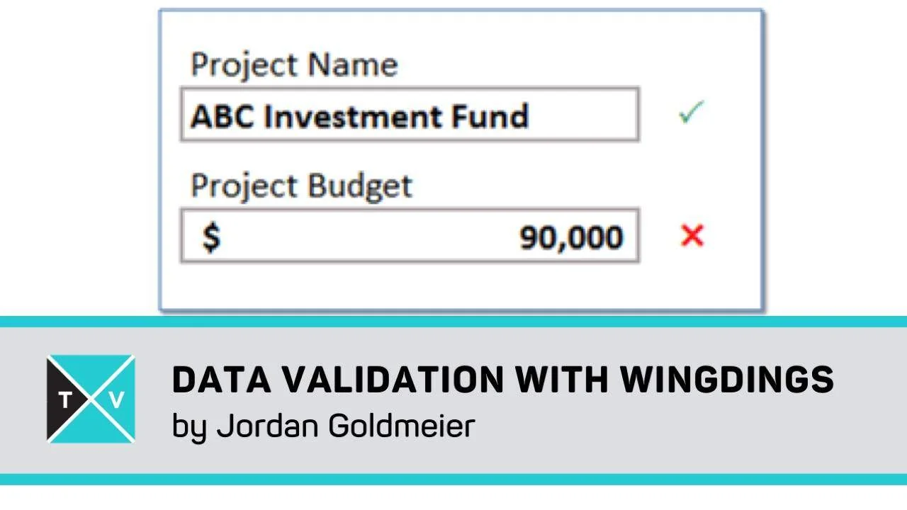
The picture below shows what you could potentially end up with. Yes, this is in Excel, and the check and cross marks are dynamic.

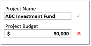
The first step is very simple. Enter a formula based on your input cells that will return TRUE or FALSE. For example, the green tick actually sees if the ‘Project Name’ is four characters long or not. Similarly, the cross checks if the ‘Project Budget’ is a number above $100,000.

You guessed it right! We will convert those TRUE and FALSE into green checks and red crosses, respectively.

2 – Trick 1

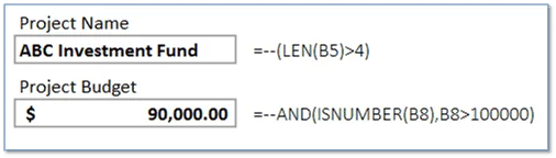
This trick is extremely simple, yet very people know about it. If a formula in a cell yields TRUE or FALSE, just wrap it in brackets and put “–“ outside. Yes, that’s a double minus. What it does is that it will convert TRUE to 1 and FALSE to 0. For example, observe the image below.

Alternatively, you can simply write an IF function which returns a 1 or a 0 instead if this trick doesn’t seem to stick with you.

3 – Trick 2

‘Custom’ format these cells and type the following:

[Color50][=1]”P”;[Color3][=0]”Д

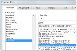
An illustration is shown in the picture.

You might be wondering what these “P” and “Д have to do with everything. The answer is very simple: once you have applied this format, select the cells and choose their font to be ‘Wingdings 2’. Yes, these two letters represent a check and a cross, respectively, in this font.

Excel Wingdings Explained

There might be two more questions lingering around still. We will answer those here.

What are these “Color50” and “Color3” doing?
It is a little known fact that one can specify color the text within a cell should take within ‘Custom’ format. This is exactly what “Color50” (green) and “Color3” (red) are doing. Note that this is also why we do not need to use Conditional Formatting for your checks and crosses.

How did we get “P” and “Д?
These symbols under ‘Wingdings 2’ translate to a check and a cross. To use other symbols, the procedure is very simple:

Just go under ‘Insert’ tab and select ‘Symbol’. Now select ‘Wingdings 2’ from the dropdown menu and browse through symbols you like. When you find them, select them and click on ‘Insert’. Once you are done, just select the cell where you inserted these symbols and set a regular font (such as Calibri).

Now you can use the regular version of the symbols you liked instead of P or Ð.

What’s next?

What Jordan taught us is actually very cool. Practice these out! If you add your own personal touches to it, be sure to share it with us in the comments section below.

And do not forget to share this “awesomeness” with your friends and colleagues.