Numbering Grouped Data for Pivot Tables

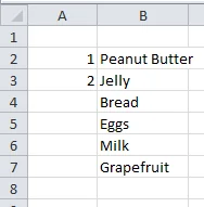
We’ve all had some experience with Excel’s automatic numbering.  For example, if you have a simple list and you would like to add consecutive numbers to a column next to your data, you’d simply select the cells containing your first two numbers and then drag accordingly.  Take a look at the sheet below to see an example.

!

But real-world lists aren’t always so simple.  And for certain data, a simple consecutive list just won’t do.  Sometimes we receive spreadsheets that have some type of intrinsic grouping but no unique group identifier. The challenge is that we would really like to apply Pivot Tables to this data, but we can’t do anything until there exists some type of group identifier.

Problem #1: Items grouped without collation
Take a look at the datasheet below from my nonexistent accounting information system.

!

Because I’m smart(ish), I know that a new group begins every third row of data.  The first three rows of data (Excel rows 2,3, and 4) represent store 1, the next three store 2, and so forth.  I would like to add an additional group_id column such that each grouping is numbered consecutively.  Something like this:

!

How?  I use this formula, 

=INT((ROW()-2)/3) + 1

Then fill downward.  This works by applying integer division in the amount of each item in a group to the current row. So, for row 3, we have 

=INT((ROW()-2)/3) -> =INT((3-2)/3) – > =INT(1/3) -> = INT(0.33) = 0.  

(If it’s been a while since your last algebra class, just think of it as dividing and then “rounding down” the result.)

I add one (“+ 1”) at the end of the formula so that my grouping doesn’t start at zero.  That’s optional.

Notice though, that I subtract 2 because my data starts on row 2.  If I had started on row 1, I would likewise subtract 1; for row 3, subtract 3.  Here’s a cheat sheet:

For Items Grouped Without Collation

=INT**((ROW()-First row of data on spreadsheet) / # Items per Group)****[+1] optional**  

Problem #2: Items grouped with collation

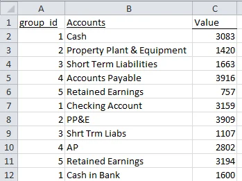
In the following spreadsheet, we’ve culled information from many different spreadsheets maintained by many different people.

!

The problem is that each spreadsheet administrator used a different naming convention for the same account (see the highlighted accounts).  And take a look at the final Retained Earnings and note that it is labeled ”  RE.”  Those extra spaces can creep into the spreadsheet and easily go unnoticed.  What a nightmare.

But wait, our list has some semblance of order: accounts can be grouped every sixth row. We just need to group each item, one through five, until the end of the list.  Like so,

!

How?  With this formula,

=MOD(ROW() – 2,5) + 1

This should look familiar to the one above.  But instead of using integer division, we’re now using modulo division; that is, we’re interested in the remainder.  Take row 3

=MOD(ROW()-2, 5)+1 ->  =MOD(3-2, 5)+1  – >  =MOD(1, 5)+1  -> = 1+1 =2.

Here’s the cheat sheet:

For Items Grouped With Collation

=MOD**((ROW()-First row of data on spreadsheet,# Items per Group)****[+1] optional**  

Final Thoughts

1.  Once you’ve created your new group_id column, it’s a good idea to select your new work, copy, and then paste as values.  If the groupings aren’t going to change later, there’s no reason to keep it as a formula.  Remember, fewer formulas means better Excel performance — especially if you plan to use a Pivot Table later.

2.  If you’re not into the numbering scheme, create a lookup table that maps the numbers to a proper name.  Create another column at the front of your data and use a lookup method, like Index, to map the correct names.  Then do a copy/paste values.

3. If you have a list scheme you use quite often, you can actually save it as a custom fill series and then use it later.

Remember:

For Items Grouped Without Collation

=INT**((ROW()-First row of data on spreadsheet) / # Items per Group)****[+1] optional**  

For Items Grouped With Collation

=MOD**((ROW()-First row of data on spreadsheet,# Items per Group)****[+1] optional**